MRD: Using Physically Based Differentiable Rendering to Probe Vision Models for 3D Scene Understanding

TL;DR
The idea of model metamers such as in Feather et al. 2023^[?] is what we extend with physically based differentiable rendering. We explore sensitivities and invariances of vision models by probing them to reconstruct certain physical scene parameters. This can provide a hint in what features a network actually encodes while learning on 2D images.

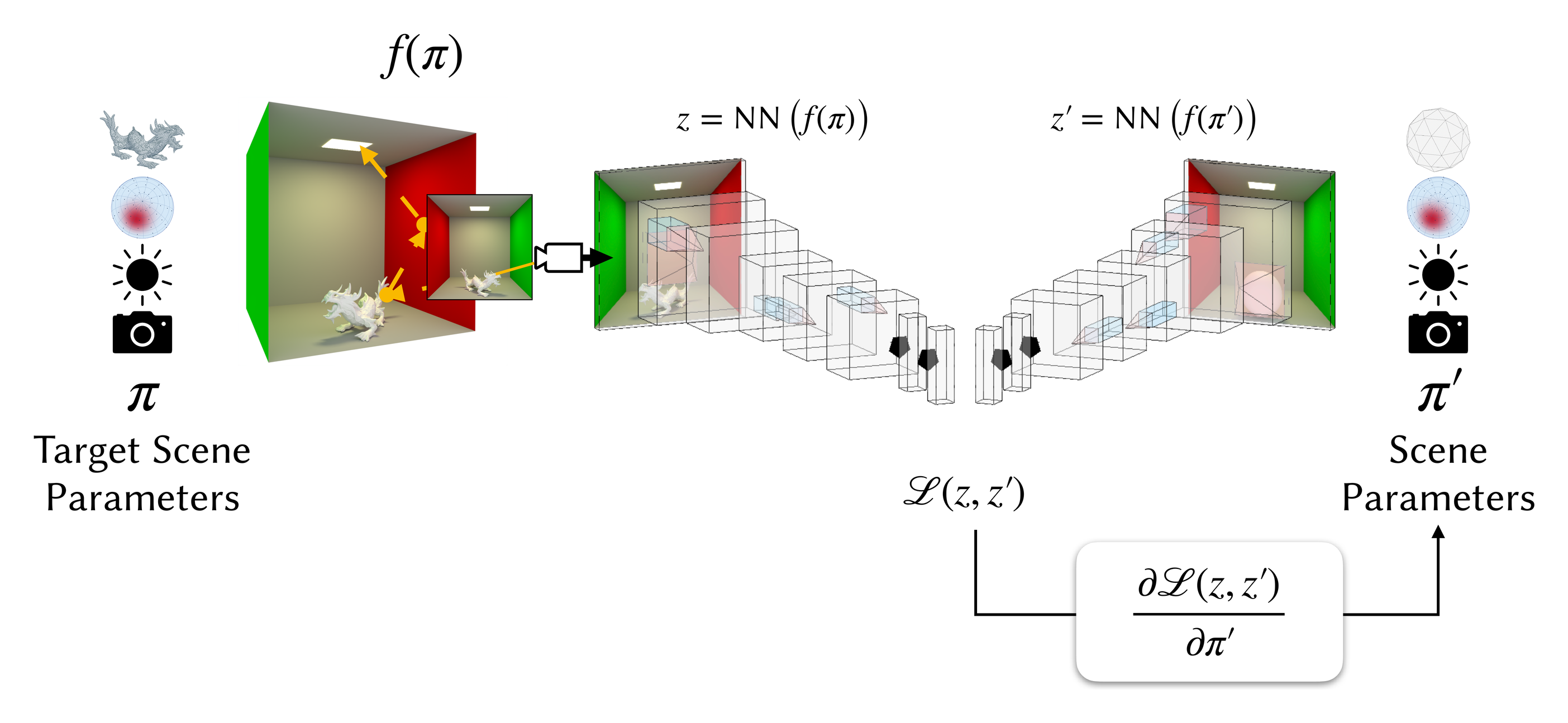
MRD: probing vision models’ implicit 3D scene understanding by optimising physical scene parameters, rather than pixels, to find model metamers.

Model metamers — but physically based.

Metamers are visual stimuli that appear the same even if the underlying cause is differnet. There is a long history on the study of metamers and what they can tell us about the human/machine perception, because of that exact property revealing invariances.

A common example is the spectra, where an object appears the same colour under different lights, to statistical metamers which compute some image statistics and further optimises a plain image to fulfill the image statistics, over to model metamers, which test the idea of finding different inputs to a neural network producing the same activation in the network’s latent space.

Wouldn’t it be cool to probe neural networks directly for different parameters and see what invariances they show? This is what led us to the idea to extend model metamers and instead of optimising an image directly, we optimise the scene description that produces the image. This grants us the added benefit of a physical-plausible space and direct control over the parameters, i.e., one can only change a single parameter of interest (surface roughness) and find configurations producing the same activation for it.

Physically Based (Differentiable) Rendering in a Nutshell

Rendering is the process of image synthesis, i.e., a function that maps a set of scene parameters onto the 2D image space. The scene parameters describe the lighting, the objects’ shape along their materials, potential media and the camera parameters from which we view the scene.

There are a couple of different possibilities to synthesise an image. We are interested in physical-plausibility and therefore want to simulate light transport properly — using path tracing. The idea of path tracing is simple, we follow the light from the camera to the light source (because we know that light will hit the camera sensor, so tracing from the light source will just waste a lot of effort). The pixels will be accumulated on the film, our 2D image.

From the camera sensor to the light source, the light usually interacts with multiple objects. Each object has a surface which will impact how light will be propagated throughout the scene. When light intersects with a surface we evaluate the bidirectional scattering distribution function (BSDF) which computes the amount of light reflected of the surface and how much light is transported through the object. Doing this only once is not sufficient to approximate the different paths that light can take, thus to find a good solution of light transport in a scene, we need to do this multiple times for each pixel, so all boils down to turning into an integration problem which we solve using Monte Carlo integration. This integrator should be ideally unbiased, so we find on average the right solution. The main bottleneck — variance — which decreases the more samples per pixel we accumulate.

Recently, a lot of research has been done on making the light transport differentiable, enabling the optimisation of scene parameters via gradient descent. This is the core idea of differentiable rendering — computing gradients with respect to some latent or scene parameters. Our framework of choice was Mitsuba 3.

A more thorough introduction to physically based differentiable rendering is available in the manuscript.

Differentiable Rendering + Neural Nets?

Now that we’ve buckled in and holistically understood what physics based differentiable rendering buys us, we need to talk about the actual experiments which involves bringing differentiable rendering and neural nets in one pipeline. Luckily this comes for free, because after you set up your scene in Mitsuba and just wrap the loss function (which involves the forward pass of the net) in a small decorator to wrap the gradient tape in Dr.Jit’s. If you are interested in this part, please consult the modelling module in my implementation.

Ways to build your scene

So, we’ve now implemented the model and the forward pass to the layer you want to probe. Now we need to talk about our scene. A scene in Mitsuba is either defined by XML file(s), or using Python’s dictionary format. I got lazy at some point and build a parser for the documentation which allows you to build your scenes programmatically in Python (with autocompletion and docs build in). Another modern way to author scenes is via OpenUSD. This comes with Delio and colleagues’ implementation of a Hydra backend: hdMitsuba. hdMitsuba also comes with a tool converting OpenUSD scenes to Mitsuba compatible scenes. This comes with its own set of problems, i.e. building OpenUSD and some elements are not supported yet in Mitsuba. The scene in our case is a very simple setup: a single geometry centered and lit via an environment map. While I am aware that this does not reflect the real world nor the training data diet of the models we probe, it should still be possible — and in fact, it is possible — to gain some findings from such as scene.

Way too many GPU hours to burn

While a scene has a vast amount of parameters, I decided the best way to go about introducing this new method is to reproduce findings from earlier work such as Geirhos et al.^[?] and Feather et al.^[?] and thus using similar networks as they did. In total we used six networks spanning from traditional CNNs such as ResNet50 and its shape biased twin ResNet-SIN over to perceptual losses including LPIPS (VGG) and VGG (the same backend as LPIPS) and finally testing newer models as DINOv2 and CLIP.

The challenge is mostly an engineering problem here, because if you don’t have sufficient VRAM, you will need to think about how to fit both the network and the renderer onto a single card. The used memory both depends on the Mitsuba integrator used and the length of your light paths. Picking wisely is not obligatory here. I easily had situations in where I was running OOM on a 48 GB VRAM card, just because I used an integrator I didn’t need to use, because I was not solving for e.g. translucency. In theory, you could use multiple GPUs, but IPC is painfully slow for moving gradients between processes. Yet there is one thing that could work out — dlpack. dlpack is a tensor structure that sits in-memory and can therefore be shared between frameworks for example it enables Mitsuba and PyTorch interop. One could use this to share the tensors/gradients from device to device.

Apart from the VRAM issues, we also have another problem involving differentiable rendering — variance. Variance really can kill the optimisation and leads to a ton of local minima in which we can land. This can only be tackled with more samples per pixel, which also increase the amount of VRAM required for the optimisation process. A promising paper introduces radiance caching^[?] to reduce the variance with a balancing weight where the radiance cache becomes useful and where not. I did not test this in our approach, but I am happy to hear about people who tried it.

We test two scenarios: (1) shape reconstruction and (2) material reconstruction.

Triangle madness

Shape reconstruction is tricky. An object in computer graphics is primarily modelled using triangulated meshes (because smallest entity that can depict a surface and the GPU can process them very quickly). Mesh optimisation is very prone to ill-conditioned gradients and while this makes it not already painful enough, changing vertices and the shape of objects introduces discontinuities in the integration problem. Not handled properly, this will lead to wrong gradients — and up to today, this is an active research area in differentiable rendering.

To deal with the discontinuities in the shape optimisation a projective integrator^[?], sampling the borders by changing the integration domain instead of the integrand itself. I managed to recover the meshes by trying around different $\lambda$ regularisations, because the original Large Steps^[?] paper used a pure PyTorch backend for the reconstruction, which makes it behave differently from running it with an actual differentiable renderer.

There’s more recent work^[?] on this mitigating some of the issues with the Large Steps approach, but we found it to work against our current pipeline which were non-negotiable. Happy to see people tackling this. In the end, a good initalisation may already help wonders.

Material reconstruction is bliss

Contrary to the shape reconstruction, material was a tad easier to tackle. Material more or less boils down to a texture problem with the additional constraint of finding the right optical parameters.

We usually start our search from a Principled BSDF, or more precisely — a Disney BSDF. It can model a broad range of materials and most of the parameters can be textured. The reconstruction problem is somehow similar as a look development artist would approch the design of a new material, but with very limited knobs. The truth is, most materials in VFX and the real world are layered. They are out of question for now, and we may rather try to reconstruct textured parameterisations such as anisotropy, metalness or the albedo.

Besides recovering translucency, this was a rather trivial problem, because we didn’t need to use the path tracing integrator which was quite hacky with VRAM limitations.

Translucency is the one case where the two outcomes — finding a metamer, and recovering the actual material — visibly split. Below, both VGG’s and CLIP’s optimisation tracks the pixel-space baseline closely enough to count as a metamer, but if you watch the reconstruction converge you’ll see it never regains the light transmission of the target; it settles on an opaque, textured stand-in instead.

Findings

First we need to get the elephant out of the room; there is no single metric that can determine if we are metameric or not. This was absolutely mental, because going back and forth finding a suitable way to present the results without biasing them — was no easy feat. After a couple of rounds in review at NeurIPS and Journal of Vision, the final conclusion was, we try to make the results informative and as readable as possible. Instead of just evaluating and reporting the $\ell_{2}$-normalised cosine similarity, we also computed correlations, similarities and a Bayes factor whenever possible.

Baseline scores

To have something comparable we ran all experiments with pixel-based loss functions which usually worked quite well. The reconstruction steps were passed through all six networks to compute the latent spaces which were used to compute the baseline scores. This meant, we only added scenes and experiments for which we could find a working baseline reconstruction using mean-absolute/squared errors.

Verdict time

Shape is hard and underdetermined and even the shape-biased net is rather allowing broad reconstructions, so the biasing more or less broadening the space of invariances. For material, we can work with strong inductive biases for BSDF parameters. Lower layers, yielding more photometric information (no latent space mash-up of convolved pixels) work well with shape and textures. This becomes apparent looking at the results of VGG and LPIPS which accumulate layer-wise information for the final latent. ResNet50’s earlier layers also show the same behaviour.

The best statement so far on this:

If any of these models represent what our visual system is doing, it would not matter what shape/material would come out of it, because if I ask you to think of a dragon you will think of a dragon with a shape you imagine it to be, but it would probably entails some scales, a fang and a tail — potentially it would even have wings. So the idea is, networks that are congruent with the visual system should produce any dragon, but a dragon at last.

Meshes and materials are just a small subset of parameters we can inspect. Heck, even the material experiments I ran are quite rudimentary. There are also a couple of natural ambiguities that one can check. In the end, it was a proof-of-principle and I think it was successful in that.

My strong guess is, physics based differnetiable rendering will become more relevant in vision science, because neural networks unfortunately are obscurring the knowledge further. Actually, I will dedicate my doctorate to make differentiable rendering an option in future studies and hope to provide some useful insights in the process.